Bar Chart
Bar charts should be used when you are showing segments of information. Vertical bar charts are useful to compare different categorical or discrete variables, such as age groups, classes, schools, etc., as long as there are not too many categories to compare. They are also very useful for time series data.
Quick Start
The bar chart expect the following minimum columns from data source: Value, Series, Category.
One may confuse Category and Series. Category of the bar chart are shown on the axis, such as "A", "B", "C", 2021, 2022, 2023 or even datetime 1609419600, 1612098000, 1614517200 (unix time for 2021-01-01, 2021-02-01, 2021-03-01). Series are used for color-coding and creating legend to show that the values belong to the same "series".
The following data source gives a simple bar chart:
{
  data: {
    Value: [
      1,
      2,
      3,
      4,
    ],
    Name: [
      'Series 1',
      'Series 2',
      'Series 1',
      'Series 2',
    ],
    Category: [
      'A',
      'B',
      'B',
      'A',
    ],
  },
  definitions: {
    Value: {
      kind: 'number',
      optional: true,
    },
    Name: {
      kind: 'string',
      optional: true,
    },
    Category: {
      kind: 'string',
      optional: true,
    },
  },
  version: '1.0.0',
  sddFormat: 'sdd/table/object-of-arrays',
}
After connecting the data source to bar chart. One needs to specify the mapping of columns for the chart. Category->Category, Value->Value and Name->Series.
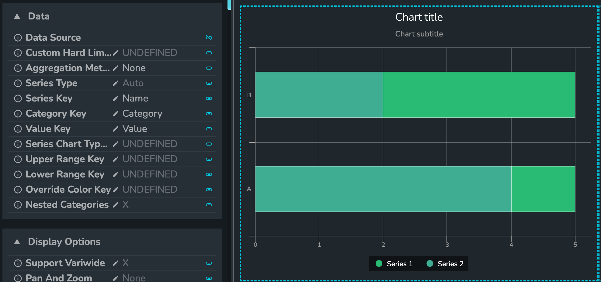
The default Bar Chart looks pretty good, but there are a few things people tend to customize.
Title and Subtitle
Title and Subtitle can be modified under the Title section under component property, alongside with the alignments.
Bar Chart Orientation
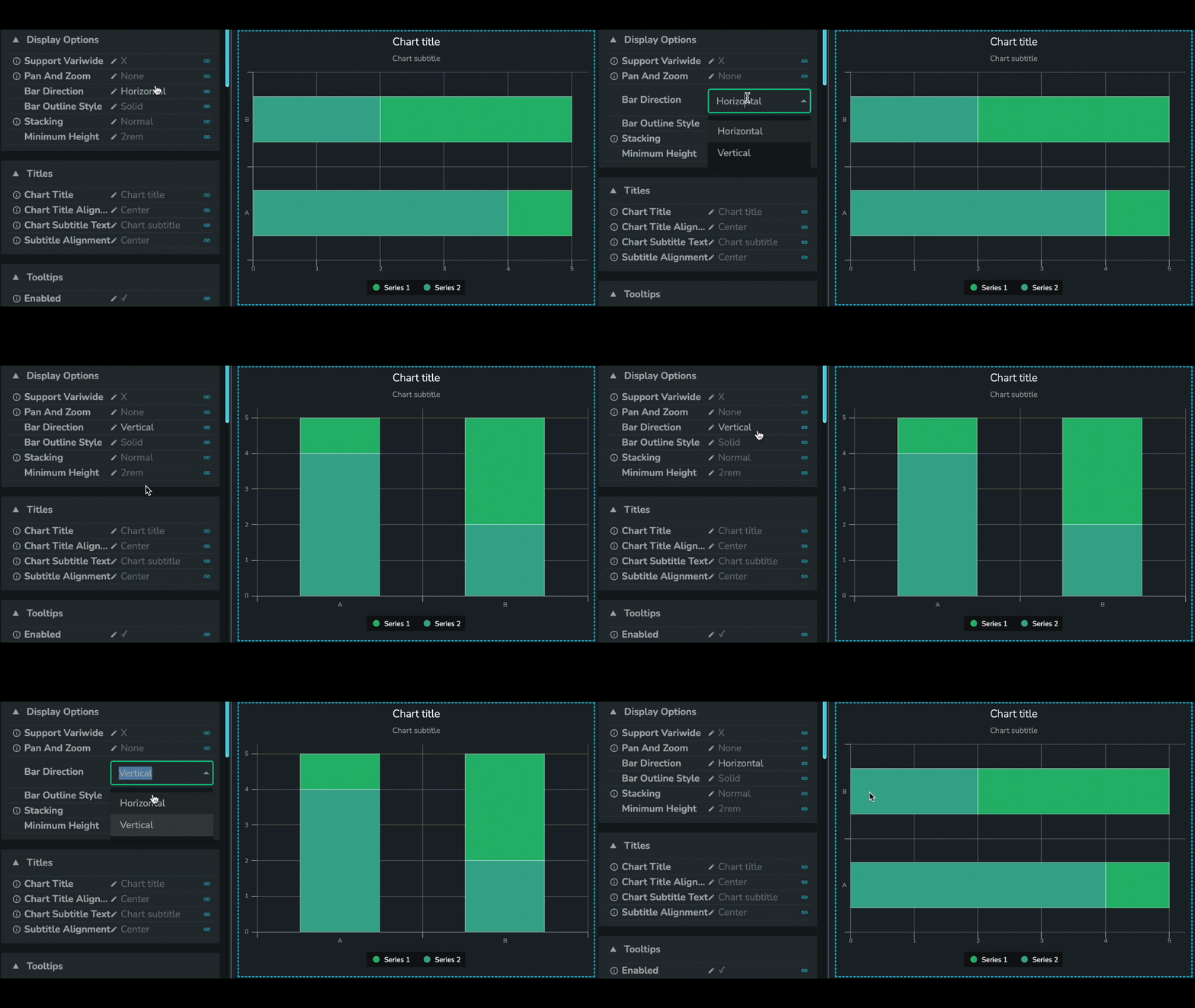
To change the orientation of the bar charts, go to Display Options->Bar Direction and pick either Horizontal or Vertical.
Custom Color
By default, the component will assign colors using series key. If custom color assignment is needed, simply add a column color with hex color code and select column color under Override Color Key under Data property.
Category Data Types
Category or x-axis takes in three types of data. Category, Numeric and Datetime.
It's worth pointing out that Datetime takes unix timestamp like 1609419600, 1612098000, 1614517200 (unix time for 2021-01-01, 2021-02-01, 2021-03-01). When Datetime is toggled on, they will be displayed as 2021-01-01, 2021-02-01, 2021-03-01 respectively.
If configuring using unix time is cumbersome, one may simply use Category with strings such as 2021-01-01 or 'Jan 2021'.
However, when using formats such as 'Jan 2021', the component will order the axis in alphabetical order, hence it may be necessary to define a custom sorting logic by adding a column in Data Source to define the desired ordering using the Sorting option under Categorical Axis property.
Aggregations
Component level data aggregation method that determines how should the data be aggregated in case there are more than one values with the same Categorical and Value axis values from the same series.
The available options are:
NoneSumCountUnique CountAverageMedianVarianceStandard DeviationPercentile(also requires the percentile specified)
Bar-Line Chart
Bar-Line charts show two metric values aggregated across a group dimension. They are useful for showing quantity alongside changes in trends over time. The first Y-axis metric displays as a bar, and the second displays as a line.
The Bar Chart component supports Bar-Line Chart mode, but it is not very obvious how to achieve it.
Here is an example of Bar-Line Chart data source. Note there is a column called plot_type that takes value 'bar' or 'line'.
{
  sddFormat: 'sdd/table/array-of-objects',
  version: '1.0.0',
  definitions: {
    year: {
      kind: 'integer',
      optional: false,
    },
    value: {
      kind: 'number',
      optional: true,
    },
    series_name: {
      kind: 'string',
      optional: true,
    },
    plot_type: {
      kind: 'string',
      optional: true,
    },
  },
  data: [
    {
      year: 2023,
      value: 565,
      series_name: 'Additional Cost',
      plot_type: 'bar',
    },
    {
      year: 2024,
      value: 628,
      series_name: 'Additional Cost',
      plot_type: 'bar',
    },
    {
      year: 2025,
      value: 250,
      series_name: 'Additional Cost',
      plot_type: 'bar',
    },
    {
      year: 2026,
      value: 300,
      series_name: 'Additional Cost',
      plot_type: 'bar',
    },
    {
      year: 2027,
      value: 455,
      series_name: 'Additional Cost',
      plot_type: 'bar',
    },
    {
      year: 2028,
      value: 470,
      series_name: 'Additional Cost',
      plot_type: 'bar',
    },
    {
      year: 2029,
      value: 650,
      series_name: 'Additional Cost',
      plot_type: 'bar',
    },
    {
      year: 2030,
      value: 750,
      series_name: 'Additional Cost',
      plot_type: 'bar',
    },
    {
      year: 2031,
      value: 880,
      series_name: 'Additional Cost',
      plot_type: 'bar',
    },
    {
      year: 2032,
      value: 987,
      series_name: 'Additional Cost',
      plot_type: 'bar',
    },
    {
      year: 2033,
      value: 1000,
      series_name: 'Additional Cost',
      plot_type: 'bar',
    },
    {
      year: 2034,
      value: 1100,
      series_name: 'Additional Cost',
      plot_type: 'bar',
    },
    {
      year: 2035,
      value: 1190,
      series_name: 'Additional Cost',
      plot_type: 'bar',
    },
    {
      year: 2036,
      value: 1270,
      series_name: 'Additional Cost',
      plot_type: 'bar',
    },
    {
      year: 2037,
      value: 1361,
      series_name: 'Additional Cost',
      plot_type: 'bar',
    },
    {
      year: 2038,
      value: 1138,
      series_name: 'Additional Cost',
      plot_type: 'bar',
    },
    {
      year: 2023,
      value: 2729,
      series_name: 'Base Cost',
      plot_type: 'bar',
    },
    {
      year: 2024,
      value: 2529,
      series_name: 'Base Cost',
      plot_type: 'bar',
    },
    {
      year: 2025,
      value: 2294,
      series_name: 'Base Cost',
      plot_type: 'bar',
    },
    {
      year: 2026,
      value: 2926,
      series_name: 'Base Cost',
      plot_type: 'bar',
    },
    {
      year: 2027,
      value: 2152,
      series_name: 'Base Cost',
      plot_type: 'bar',
    },
    {
      year: 2028,
      value: 2938,
      series_name: 'Base Cost',
      plot_type: 'bar',
    },
    {
      year: 2029,
      value: 2801,
      series_name: 'Base Cost',
      plot_type: 'bar',
    },
    {
      year: 2030,
      value: 2890,
      series_name: 'Base Cost',
      plot_type: 'bar',
    },
    {
      year: 2031,
      value: 3000,
      series_name: 'Base Cost',
      plot_type: 'bar',
    },
    {
      year: 2032,
      value: 2629,
      series_name: 'Base Cost',
      plot_type: 'bar',
    },
    {
      year: 2033,
      value: 2430,
      series_name: 'Base Cost',
      plot_type: 'bar',
    },
    {
      year: 2034,
      value: 2629,
      series_name: 'Base Cost',
      plot_type: 'bar',
    },
    {
      year: 2035,
      value: 2648,
      series_name: 'Base Cost',
      plot_type: 'bar',
    },
    {
      year: 2036,
      value: 4639,
      series_name: 'Base Cost',
      plot_type: 'bar',
    },
    {
      year: 2037,
      value: 1947,
      series_name: 'Base Cost',
      plot_type: 'bar',
    },
    {
      year: 2038,
      value: 3019,
      series_name: 'Base Cost',
      plot_type: 'bar',
    },
    {
      year: 2023,
      value: 2500,
      series_name: 'Revenue',
      plot_type: 'line',
    },
    {
      year: 2024,
      value: 2336,
      series_name: 'Revenue',
      plot_type: 'line',
    },
    {
      year: 2025,
      value: 2514,
      series_name: 'Revenue',
      plot_type: 'line',
    },
    {
      year: 2026,
      value: 2506,
      series_name: 'Revenue',
      plot_type: 'line',
    },
    {
      year: 2027,
      value: 2860,
      series_name: 'Revenue',
      plot_type: 'line',
    },
    {
      year: 2028,
      value: 2163,
      series_name: 'Revenue',
      plot_type: 'line',
    },
    {
      year: 2029,
      value: 2900,
      series_name: 'Revenue',
      plot_type: 'line',
    },
    {
      year: 2030,
      value: 2999,
      series_name: 'Revenue',
      plot_type: 'line',
    },
    {
      year: 2031,
      value: 3333,
      series_name: 'Revenue',
      plot_type: 'line',
    },
    {
      year: 2032,
      value: 3190,
      series_name: 'Revenue',
      plot_type: 'line',
    },
    {
      year: 2033,
      value: 3389,
      series_name: 'Revenue',
      plot_type: 'line',
    },
    {
      year: 2034,
      value: 3390,
      series_name: 'Revenue',
      plot_type: 'line',
    },
    {
      year: 2035,
      value: 3514,
      series_name: 'Revenue',
      plot_type: 'line',
    },
    {
      year: 2036,
      value: 3649,
      series_name: 'Revenue',
      plot_type: 'line',
    },
    {
      year: 2037,
      value: 3729,
      series_name: 'Revenue',
      plot_type: 'line',
    },
    {
      year: 2038,
      value: 3967,
      series_name: 'Revenue',
      plot_type: 'line',
    },
    {
      year: 2023,
      value: 2500,
      series_name: 'Net Revenue with Projects',
      plot_type: 'line',
    },
    {
      year: 2024,
      value: 3000,
      series_name: 'Net Revenue with Projects',
      plot_type: 'line',
    },
    {
      year: 2025,
      value: 3000,
      series_name: 'Net Revenue with Projects',
      plot_type: 'line',
    },
    {
      year: 2026,
      value: 3218,
      series_name: 'Net Revenue with Projects',
      plot_type: 'line',
    },
    {
      year: 2027,
      value: 3319,
      series_name: 'Net Revenue with Projects',
      plot_type: 'line',
    },
    {
      year: 2028,
      value: 3427,
      series_name: 'Net Revenue with Projects',
      plot_type: 'line',
    },
    {
      year: 2029,
      value: 3609,
      series_name: 'Net Revenue with Projects',
      plot_type: 'line',
    },
    {
      year: 2030,
      value: 3799,
      series_name: 'Net Revenue with Projects',
      plot_type: 'line',
    },
    {
      year: 2031,
      value: 3201,
      series_name: 'Net Revenue with Projects',
      plot_type: 'line',
    },
    {
      year: 2032,
      value: 4219,
      series_name: 'Net Revenue with Projects',
      plot_type: 'line',
    },
    {
      year: 2033,
      value: 4205,
      series_name: 'Net Revenue with Projects',
      plot_type: 'line',
    },
    {
      year: 2034,
      value: 4486,
      series_name: 'Net Revenue with Projects',
      plot_type: 'line',
    },
    {
      year: 2035,
      value: 4144,
      series_name: 'Net Revenue with Projects',
      plot_type: 'line',
    },
    {
      year: 2036,
      value: 5101,
      series_name: 'Net Revenue with Projects',
      plot_type: 'line',
    },
    {
      year: 2037,
      value: 5729,
      series_name: 'Net Revenue with Projects',
      plot_type: 'line',
    },
    {
      year: 2038,
      value: 5004,
      series_name: 'Net Revenue with Projects',
      plot_type: 'line',
    },
    {
      year: 2023,
      value: 2711,
      series_name: 'Original Net Revenue',
      plot_type: 'line',
    },
    {
      year: 2024,
      value: 2862,
      series_name: 'Original Net Revenue',
      plot_type: 'line',
    },
    {
      year: 2025,
      value: 2316,
      series_name: 'Original Net Revenue',
      plot_type: 'line',
    },
    {
      year: 2026,
      value: 2987,
      series_name: 'Original Net Revenue',
      plot_type: 'line',
    },
    {
      year: 2027,
      value: 3002,
      series_name: 'Original Net Revenue',
      plot_type: 'line',
    },
    {
      year: 2028,
      value: 3229,
      series_name: 'Original Net Revenue',
      plot_type: 'line',
    },
    {
      year: 2029,
      value: 3339,
      series_name: 'Original Net Revenue',
      plot_type: 'line',
    },
    {
      year: 2030,
      value: 3458,
      series_name: 'Original Net Revenue',
      plot_type: 'line',
    },
    {
      year: 2031,
      value: 3549,
      series_name: 'Original Net Revenue',
      plot_type: 'line',
    },
    {
      year: 2032,
      value: 3686,
      series_name: 'Original Net Revenue',
      plot_type: 'line',
    },
    {
      year: 2033,
      value: 3819,
      series_name: 'Original Net Revenue',
      plot_type: 'line',
    },
    {
      year: 2034,
      value: 3995,
      series_name: 'Original Net Revenue',
      plot_type: 'line',
    },
    {
      year: 2035,
      value: 3997,
      series_name: 'Original Net Revenue',
      plot_type: 'line',
    },
    {
      year: 2036,
      value: 5032,
      series_name: 'Original Net Revenue',
      plot_type: 'line',
    },
    {
      year: 2037,
      value: 5463,
      series_name: 'Original Net Revenue',
      plot_type: 'line',
    },
    {
      year: 2038,
      value: 6858,
      series_name: 'Original Net Revenue',
      plot_type: 'line',
    },
  ],
  tableConstraints: {
    validity: 'enforced',
  },
}
The new column plot_type can be passed into Series Chart type Key under Data property and get a horizontally orientated Bar-Line Chart. At the time of writing, simple changing the orientation of bars from horizontal to vertical does not work.
The workaround for creating a vertically stacked bar-line chart is to use Manual mode under Data property. Under Manual mode, create a new entry for Series Config by clicking Add and populate values like below
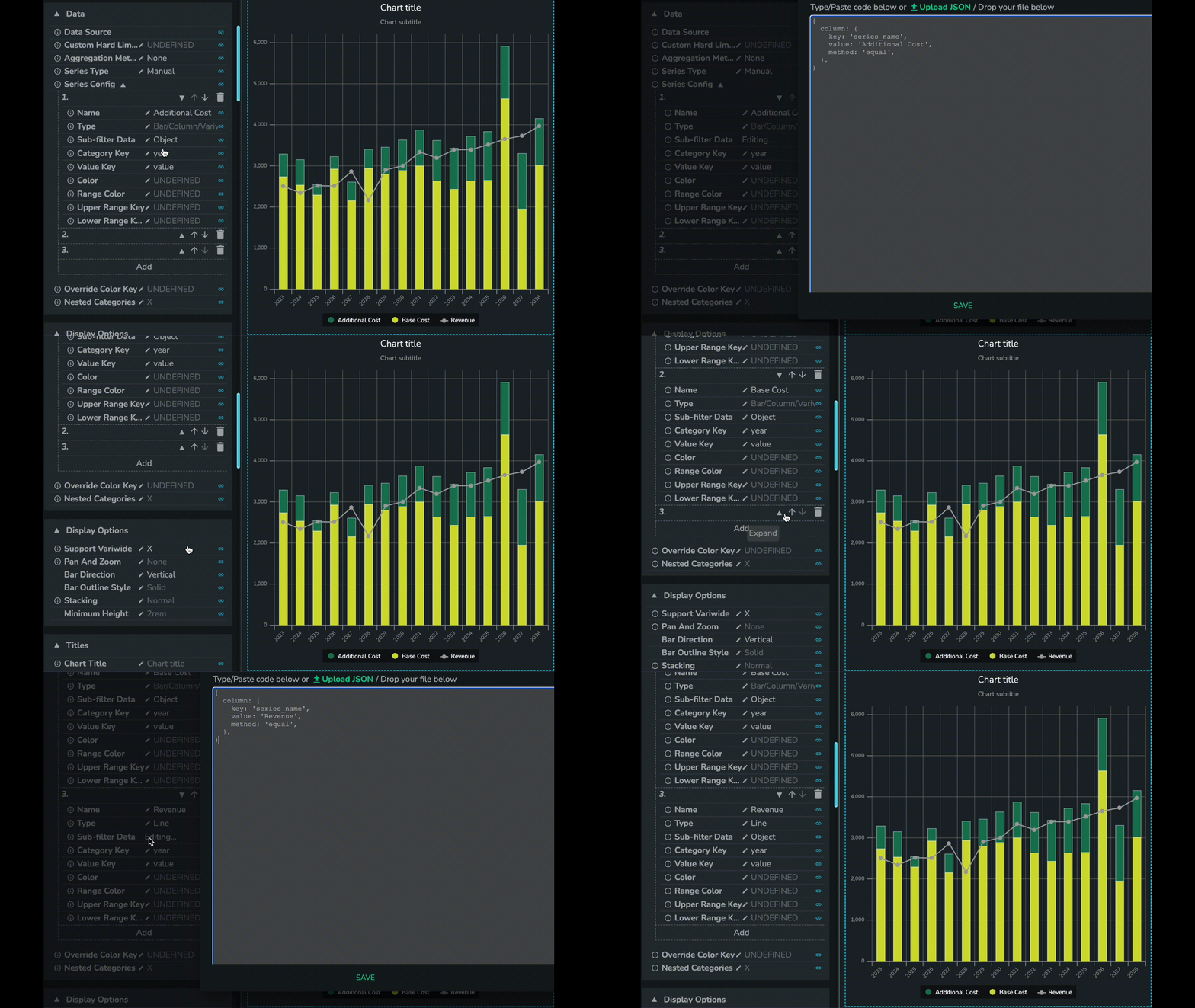
{
  column: {
    key: 'series_name',
    value: 'Additional Cost',
    method: 'equal',
  },
}
More about Bar Chart
There are more resources available for the Bar Chart component.